 |
This article is the appendix of a paper by William Gray, emeritus professor of atmospheric science at Colorado State University, on the paper titled:
On The Hijacking of the American Meteorological Society (AMS)
(Scientific Discussion)
ABSTRACT
I am presently preparing a lengthy research paper to back up my low estimates of the potential for human-induced global warming resulting from a doubling of CO2. This Appendix attempts to show that only a very small amount of the global warming that has been observed over the last century and since the mid-1970s can be attributed to global CO2 increases. A second paper with yet more scientific documentation will hopefully be ready in another couple of months.
A doubling of CO2 would lead to a global infrared (IR) energy blockage to space (all other processes held constant) of about 3.7 W/m2. We are about one-third (~1.2 W/m2) of the way to a CO2 doubling from the pre-industrial state. The balancing of the 1.2 W/m2 energy gain from CO2 increase that has so far occurred would lead to an upper tropospheric emission temperature increase of about 0.3oC and a corresponding surface temperature increase of about 0.15oC. This is less than a quarter of the ~0.7oC global temperature increase that has been observed since the start of the industrial revolution. Processes more dominant than CO2 increases had to be responsible for most of the global warming that has occurred.
The globe has continuous solar energy absorption of about 235 W/m2 which is balanced by continuous infrared (IR) energy emittance to space of 235 W/m2. This continuous in-and-out energy flux is 200 times greater than the accumulated current CO2 induced energy gain from the mid-19th century. Long period infrared and albedo energy changes resulting from naturally occurring differences in global rainfall, cloudiness, surface sensible flux, deep ocean current changes, etc. can be considerable greater than this relatively small and gradual 1.2 W/m2 global infrared energy suppression to space. Yes, increases in CO2 are causing global warming, but very little of it. Too little to justify a sizable reduction of our society’s use of fossil-fuels for the far more expensive employment of renewable energy.
This Appendix discusses how the variation in the global ocean’s deep circulation resulting from changes in the Atlantic Thermohaline Circulation (THC) and/or the associated ocean Meridional Overturning Circulation (MOC) is the likely cause of most of the global warming that has been observed since the start of the industrial revolution and the more recent global warming that has occurred since the mid-1970s. Changes of the MOC since 1995 are hypothesized to have lead to the cessation of global warming since 1999 and to the beginning of a weak global cooling that has occurred since 2001. This weak cooling is projected to go on for the next couple of decades.
1. INTRODUCTION
There are about 20 different General Circulation Model (GCM) groups around the world that have been conducting extensive numerical modeling simulations of the likely changes in global mean temperature that should be expected to occur from a doubling of atmospheric carbon dioxide (CO2) gas. Carbon dioxide has so far risen about 33 percent (to 385 ppm) over its pre-industrial values and about 15 percent during the last 30 years. It is expected that there will be a doubling of atmospheric CO2 by the latter part of the 21st century. Most of these GCM simulations indicate that there will be a 2-5oC (4-9oF) increase in global mean temperature by the time this doubling takes place if there is no action to reduce these CO2 increases. Such large warming would cause great changes in human society. These large warming scenarios are highly unlikely, however. The GCMs greatly exaggerate the potential warming that will occur. These exaggerations are due to:
- Models assuming that an increase in atmospheric CO2 will cause weak global warming and an increase in global precipitation that will lead to a large increase in upper-level water vapor and cloudiness. They simulate that this increase in water vapor and cloudiness will block large amounts of infrared radiation emitted to space. New observations by satellite and reanalysis data however, do not support these GCM model assumptions. The global warming that has occurred since the mid-1970s has been associated with a general decrease of global upper tropospheric water vapor and an increase of Outgoing Longwave Radiation (OLR) to space. These measurements are opposite to what the models predict.
- GCMs do not currently model (or if they do – not accurately) the globe’s deep-water ocean circulation. Accurately modeling the global ocean’s deep circulation is fundamental to any realistic understanding of global temperature change. Such global deep water circulation patterns appear to be the primary control of global surface temperature. The global warming we have seen since the mid-1970s and over the last 100 years is largely due to reductions in the rate of global ocean deep water circulation (or Meridional Overturning Circulation – MOC) which is viewed as being driven by global ocean salinity variations. CO2 changes play no role in these ocean changes.
2. OTHER GCM PROBLEMS
Small-Scale Problems. In order to integrate over the entire globe and many years into the future it is necessary that the GCMs have rather large grid spacing. This requires that the GCMs employ sub-grid scale cumulus parameterization schemes which can often be poor approximations of the real-world complex, non-linear small-scale cumulus convective processes. An important deficiency in the global models is the large amount of compensating up-and-down motion occurring between grid spaces that cannot be explicitly resolved by the models (Figure 1). These poorly-resolved approximations of sub-grid scale processes are integrated by the models for hundreds of thousands of time steps into the future. This guarantees large errors. Realistic sub-grid scale parameterization schemes have yet to be developed. Most GCM modelers are unfamiliar with the detailed functioning of the hydrologic cycle. Their models assume that changes in lower and upper tropospheric water vapor occur simultaneously which the observations do not verify (Figure 2). Observations show, in fact, that as global warming has occurred since the mid-1970s that lower tropospheric water vapor has increased while upper tropospheric water vapor has decreased. This appears to be a result of there being somewhat more deep Cb convection and a higher rainfall efficiency when the globe is warmer than when it is colder. There are slightly more deep convection updrafts and compensation mass subsidence drying during times when the globe is warmer.
Much research on the small scale parameterization of cumulus convection in terms of the large scale circulation patterns was done in the 1970s and 1980s without satisfactory resolution. The topic was too complex to be resolved during this period. To move forward the GCM models primarily ignored this difficult task. They chose not to get ‘down-in-the-trenches’ on such a complex topic. They accepted a few simple compromised schemes (with known problems) and went forward with their broader-scale modeling integrations assuming that their sub-grid schemes were ‘good enough’ or that the errors would average out in the end. But the sub-grid scale approximations they have used have not been good enough and the sub-grid parameterization errors do not average out over the long integration periods.
There are many large and complicated variations as to how sub-grid scale cumulus parameterization should be accomplished with respect to differences in latitude, land, sea, season, and other conditions. There are no general sub-grid parameterization schemes that can perform this function within the various global regions and on the long climate time-scales. And there will likely never be a satisfactory scheme.
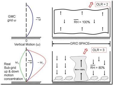
Figure 1. Idealized portrayal of how the grid size of the GCMs is too large to accommodate real sub-grid scale vertical motion. GCMs cannot resolve (top) the concentrated rain or the surrounding cloud downdrafts and subsidence within the scale of its grid space (bottom). The top and bottom diagrams contrast the mean vertical motion of the GCM (top) and the real up-and-down vertical motion of nature if deep convection is occurring within a grid space. Note that the unresolved vertical motion of the top diagram allows less OLR to escape to space – than the bottom actual representation.
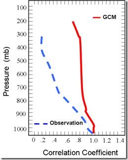
Figure 2. Comparison of correlation coefficient between upper and lower level tropospheric water vapor of the typical GCMs model output (red) and that of the Rawinsonde-reanalysis observations (blue line). The GCM model outputs are programmed to have a simultaneous moistening of the lower and upper tropospheric levels, but the observations of upper vs. lower troposphere moisture shows little correlation. This high correlation of the models causes them to artificially moisten the upper troposphere and block too much OLR to space. Adapted from Sun and Held 1996.
The net effect of the GCM’s sub-grid scale parameterization schemes is to underestimate sub-grid subsidence drying, and to unrealistically suppress OLR to space. This is one of the ways the GCMs are able to develop their large amounts of artificial warming. It is thus not so surprising that the GCMs produce so much global warming (~2 to 5oC) for only a relatively small increase (3.7 W/m2) of suppressed radiation to space for a doubling of CO2.
It is expected that global rainfall will increase somewhat as human-induced greenhouse gases increase. This increased rainfall is expected to primarily manifest itself in small amounts of increased and concentrated deep cumulus convection and increased rainfall efficiency in the normal areas where deep convection and rainfall are already occurring. This somewhat greater and more concentrated rainfall will not bring about global upper-level water vapor and cloud increase anywhere near as much as the GCM modelers have assumed. The diagram of Figure 3 gives the author’s concept of how the globe will handle a doubling of CO2 by the end of the 21st century. We will not see a global warming of 2-5oC as the GCM models indicate but rather a much more modest warming of about 0.3-0.5oC.
Albedo Considerations. Analysis of OLR and albedo from the new ISCCP (International Satellite Cloud Climatology Project – 1984-2005) for differing reanalysis determined rainfall amounts shows that at the places and times where rainfall increases that albedo goes up more than OLR goes down. There is thus more net short and long wave energy going to space in periods of increased rainfall than with decreased rainfall conditions. These observations do not agree with the programmed physics within the GCMs.
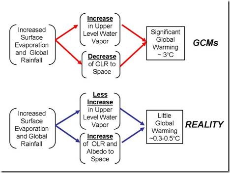
Figure 3. A view of the physical process differences between the global warming for a doubling of CO2 from the GCM climate models and reality.
Positive Water Vapor Feedback. Most geophysical systems react to forced imbalances by developing responses which oppose and weaken the initial forced imbalance; hence, a negative feedback response. Recent GCM global warming scenarios go counter to the foregoing in hypothesizing a positive feedback loop. This positive water vapor feedback assumption allows the small initial warming due to human-induced CO2 increases to be unrealistically multiplied 3-5 or more times. As AGW gases increase it does not follow that upper-level water vapor and cloudiness will increase very much. Observations indicate that the specific humidity and relative humidity of the middle and upper troposphere has been going down over the last 4-5 decades (Figure 4). The assumed positive water vapor increase with temperature as programmed into the GCM models does occur however at the surface and the lower troposphere. But this simultaneous increase of temperature and water vapor is not found in the upper troposphere near the radiation emission level. It is not the total precipitable water which is most important (measurements show this goes up with temperature) but rather the amount of water vapor near the upper tropospheric emission level which is important. This specifies the amount of infrared energy going to space.
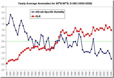
Figure 4. The NOAA-NCEP reanalysis of standardized anomalies of 400 mb (~7.5 km altitude) water vapor content (i.e. specific humidity – in blue) and Outgoing Longwave Radiation (OLR) from 1950-2008. Note the downward trend in moisture and the upward trend in OLR.
Faulty Reasoning Behind Climate GCMs. A basic assumption error behind the global GCMs has been the model builder’s general belief in the physics of the National Academy of Science (NAS) 1979 study – often referred to as The Charney Report. This report hypothesized that a doubling of atmospheric CO2 would bring about a general warming of the globe’s mean temperature between 1.5 – 4.5oC (or an average of ~ 3.0oC). This was based on the report’s assumption that the relative humidity (RH) of the atmosphere should be expected to remain quasi-constant if the globe’s temperature were to increase. The fundamental law of the Clausius-Clapeyron (CC) equation specifies that as the temperature of the air rises its ability to hold water vapor goes up exponentially. If relative humidity (RH) were to remain constant as atmospheric temperature rose then the water vapor (q) amount in the atmosphere would accordingly rise (Figure 5 and Figure 6). Observations show that this is indeed a valid assumption for the lower tropospheric levels but does not observationally apply in the upper troposphere (300-400 mb) where water vapor and relative humidity have been observed to slightly decrease as the atmospheric temperatures rises. Lower RH and reduced water vapor contents near the upper radiation emission level will act to increase the amount of outgoing longwave radiation (OLR) which will be emitted to space. By contrast, the GCMs have programmed a reduction of OLR for rising upper level temperature.
The global general circulation models (GCMs) which test the influence of CO2 increases, have accepted the hypothesized NAS – Charney Report (1979) scenario. Some of the GCM modelers such as the early NASA-GISS (Hansen 1988) model have even gone further than the Clausius-Clapeyron equation would specify for water vapor increasing with temperature. Hansen’s early GISS model assumed that a doubling of CO2 would cause the upper tropospheric RH not just to stay constant but to actually increase. And his assumed upper tropospheric increase of water vapor (q) for a doubling of CO2 led to a water vapor increase (∆q) in the upper troposphere of as much as an extremely unlikely 50 percent. These large vapor increases caused Hansen to require that his model have a tropical (30oN-30oS) upper tropospheric warming for a doubling of CO2 as much as 7oC (Figure 8). No wonder Hansen got such high values of global warming for a doubling of CO2. This logically followed from his extremely high water vapor assumptions.
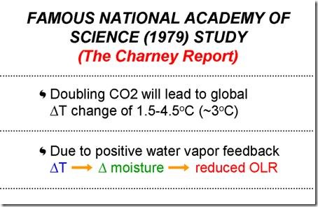
Figure 5. The very influential NAS report of 1979 which deduced that any warming of the globe would occur with near constant relative humidity (RH). Global warming consequently causes an increase in atmospheric water vapor (q) and decrease outgoing longwave radiation (OLR). This assumption appears valid in the lower troposphere but no the upper troposphere.
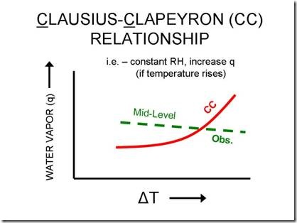
Figure 6. Clausius-Clapeyron (CC) relationship showing the required increase of water vapor as temperature increases at constant relative humidity (RH) – red line. The observations of upper tropospheric water vapor – green dashed line – do not follow this theoretical relationship. This is likely a result of a warmer climate causing more deep convection and more return flow dryer subsidence.
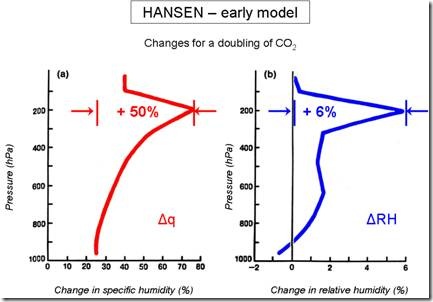
Figure 7. James Hansen’s early GISS showing his assumed increases in specific humidity (q) and RH for a doubling of CO2. Such water vapor assumptions are completely unrealistic.
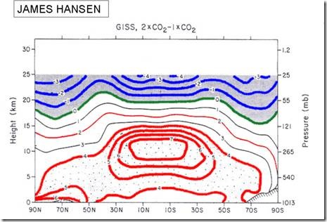
Figure 8. North-South vertical-cross section showing Hansen’s early GCM’s model change in temperature (oC) that would accompany a doubling of atmospheric CO2. There is no way a doubling of CO2 and an extra 3.7 W/m2 blockage of OLR to space could lead to such extreme upper tropospheric temperature rises. These large temperature increases occurred because of Hansen’s unrealistic upper level water vapor assumptions.
In order to obtain the global balance of incoming and outgoing radiation for his assumed high values of upper tropospheric water vapor it was necessary for Hansen to unrealistically raise his model’s upper tropospheric temperatures to obtain the amounts of Outgoing Longwave Radiation (OLR or σT4) to space that would accomplish net radiation balance. It is amazing that Hansen’s high water vapor increase assumptions for a doubling of CO2 were not immediately challenged.
It was these large amounts of warming resulting from his model’s gross over-estimate of water vapor which Hansen presented to a US Senate Committee hearing at the request of then Senator Al Gore during the hot summer of 1988. The media and much of the general public accepted it all. The environmentalists salivated. Hansen had secured his place in the sun. But history will reverse such adulation when his warming predictions are inevitable proven to be wrong.
Not only have Hansen’s extreme and unrealistic high values of upper tropospheric moisture and temperature changes (for a doubling of CO2) not been challenged, they were instead closely emulated by most of the other prominent GCM early global warming modeling groups of NOAA-GFDL (Figure 9), NCAR (Figure 10) and the British Met Service (Figure 11). They all followed suit and incorporated unrealistically high amounts of upper tropospheric water vapor and, as a result, obtained unrealistic high values of global upper and surface temperature just as Hansen had.
I am sure that the more recent global climate models of Hansen’s GISS model and the more recent, GFDL, NCAR and UKMET models have been improved. I expect the current set of GCM modelers will say I am referring to older model runs that are now obsolete. This argument does not hold however. If the more recent year models are superior to the older ones, then we would be seeing a revision downward of their warming estimates. But their newer models give much the same magnitude of warming as their older ones.
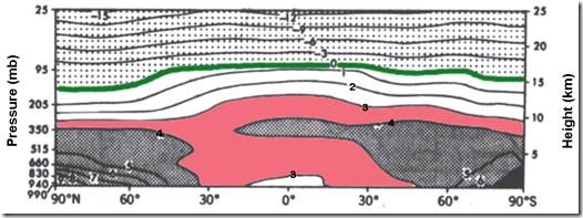
Figure 9. Same as Figure 8 but for early model NOAA-GFDL GCM temperature rises for a doubling of CO2.
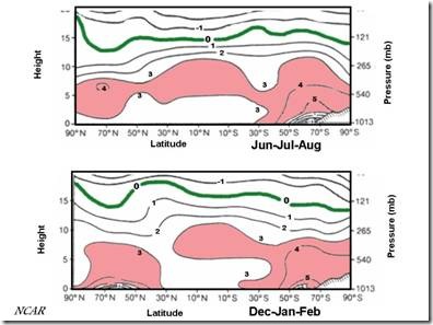
Figure 10. Same as Figure 8 but for NCAR’s early model GCM temperature rises for a doubling of CO2.


No comments:
Post a Comment